Why Miniconda and Not Just pip
Before writing a single line of Python, I spent time getting the environment right. On an M4 Mac, this matters more than on a standard x86 machine — PyTorch in particular needs the right build for Apple Silicon to use MPS (Metal Performance Shaders) for GPU acceleration. A wrongly installed torch on M4 runs on CPU only and you'll never know it.
I chose Miniconda over plain pip for one reason: environment isolation. Every project gets its own environment with its own Python version and its own package versions. When you're working across Phase 2 (ML), Phase 3 (PyTorch), and Phase 5 (LangChain), these packages can conflict badly. Conda solves that cleanly.
BFSI relevance: Banking and financial services teams run strict dependency management on every AI project. Knowing how to use conda environments is expected — it's the difference between code that runs reproducibly on a colleague's machine and code that only works on yours.
Setting Up Miniconda on M4 Mac
This is the exact sequence I ran. If you're on an M1/M2/M3/M4 Mac, use the arm64 installer specifically — not the x86 one.
# Download the arm64 installer for Apple Silicon
curl -O https://repo.anaconda.com/miniconda/Miniconda3-latest-MacOSX-arm64.sh

# Run the installer
sh Miniconda3-latest-MacOSX-arm64.sh

# Initialise conda for zsh (default shell on M4 Mac)
~/miniconda3/bin/conda init zsh

# Reload shell config
source ~/.zshrc

# Verify conda is working
conda --version
conda 24.11.1
One thing that caught me — after running conda init zsh you must restart the terminal or run source ~/.zshrc. If you skip this, the conda command won't be found.
Accepting the Terms of Service
Conda now requires explicitly accepting the Terms of Service for the default channels. Without this, package installs fail with a cryptic error:
conda tos accept --override-channels --channel https://repo.anaconda.com/pkgs/main
conda tos accept --override-channels --channel https://repo.anaconda.com/pkgs/r
Creating the AI Dev Environment
# Create a dedicated environment — Python 3.11 specifically
conda create -n ai_dev python=3.11 -y

# Activate it — you'll see (ai_dev) in your prompt
conda activate ai_dev

# Install the Day 1 libraries
pip install numpy pandas pydantic torch yfinance matplotlib

# Verify torch is using MPS (Apple Silicon GPU)
python3 -c "import torch; print(torch.backends.mps.is_available())"
True
Why Python 3.11 specifically? It's the most stable version for the full AI/ML stack in 2026. Python 3.12 has compatibility issues with some ML packages. 3.10 works but misses some modern syntax features used in newer LangChain/LangGraph code. 3.11 is the safe choice for this roadmap.
Core Python Syntax — What I Focused On
The goal today was not to master Python. It was to become comfortable reading and writing the patterns that appear constantly in data and AI work. I did not touch decorators, metaclasses, async/await, or anything complex. Those come when they're needed.
Here's what I actually wrote in basics.py — with financial data examples throughout, not generic toy examples:
# ── Variables & Data Types ───────────────────────────────
num = 3
num2 = 4
Name = "Prabhu"
age = 38

# Type conversion — useful when dealing with API responses
num_str = str(num)
print(num_str)                    # "3"
print(str(num + num2) + Name)    # "7Prabhu"
print(f"my age is {age}")        # f-strings — use these everywhere

# ── Lists — building a stock watchlist ──────────────────
stocks = []
stocks.append("AAPL")
stocks.append("TSLA")
stocks.append("MSFT")
stocks.insert(1, "HDFC")     # Indian BFSI stock at position 1
stocks.insert(2, "JIO")
stocks.append("Rakbank")
stocks.pop()                   # removes last item
stocks.pop(1)                 # removes item at index 1

print(f"stocks: {stocks}")
print(f"length: {len(stocks)}")

# Loop through watchlist
for stock in stocks:
    print(stock)

# ── Dictionaries — stock price map ───────────────────────
stock = {}
stock["AAPL"] = 200
stock["HDFC"] = 300
stock.update({"JIO": 300})

del stock["AAPL"]

# Insert at specific position (dict doesn't support insert natively)
items = list(stock.items())
items.insert(1, ("TCS", 400))
stock = dict(items)

print(f"portfolio: {stock}")
stock.clear()

# ── Functions ────────────────────────────────────────────
def greet(name):
    return f"Hello {name}"

print(greet(Name))
Why I use financial examples even for basics: When you're writing stocks.append("HDFC") instead of fruits.append("apple"), the data structure feels meaningful. BFSI hiring managers notice when your portfolio uses real domain examples from Day 1. It's a small thing that signals intent.
The Day 1 Project — AAPL Stock Analyser
This is the real output of Day 1. A script that downloads 5 years of Apple stock data, runs basic analysis, exports a CSV, and saves a price chart as a PDF. Small? Yes. But every step is real — real library, real data, real file output.
import yfinance as yf
import pandas as pd
import matplotlib.pyplot as plt

# ── Explore the Ticker object ────────────────────────────
# yf.Ticker gives you everything about one stock
stock = yf.Ticker("AAPL")

# These all work — try uncommenting one at a time
# print(stock.financials)    # Income statement
# print(stock.info)          # Company overview
# print(stock.news)          # Recent news
# print(stock.balance_sheet) # Balance sheet
# print(stock.cashflow)      # Cash flow statement
# print(stock.dividends)     # Dividend history

# ── Download historical price data ──────────────────────
data = yf.download("AAPL", start="2020-01-01")

# Uncomment to explore the data structure
# print(data.head())                    # First 5 rows
# print("Max Close:", data["Close"].max())
# print("Min Close:", data["Close"].min())
# print("Avg Close:", data["Close"].mean())

# Daily returns — how much did price change each day?
# data["Daily Return"] = data["Close"].pct_change()
# print(data["Daily Return"].head())

# ── Export to CSV ────────────────────────────────────────
data.to_csv("aapl_stock_data.csv")
print("CSV file saved successfully")

# ── Plot the close price ─────────────────────────────────
data["Close"].plot()
plt.savefig("chart.pdf", dpi=300)
# plt.show()  # Uncomment to display interactively
What Each Part Does
yf.Ticker("AAPL")
Creates a Ticker object — a Python representation of the AAPL stock. From this one object you can access financials, news, dividends, balance sheet, options chain. Everything about the company in one line. I left most of these commented out to explore — but the structure is there.
yf.download("AAPL", start="2020-01-01")
Downloads daily OHLCV data (Open, High, Low, Close, Volume) from 2020 to today as a Pandas DataFrame. This is real market data — the same data that quantitative analysts at banks work with. The result is a DataFrame with date as the index and 5 price/volume columns.
data.to_csv("aapl_stock_data.csv")
Exports the entire 5-year dataset to CSV. A tangible file output — not just a print statement. This CSV becomes the training data foundation for later phases when we build ML models on historical price data.
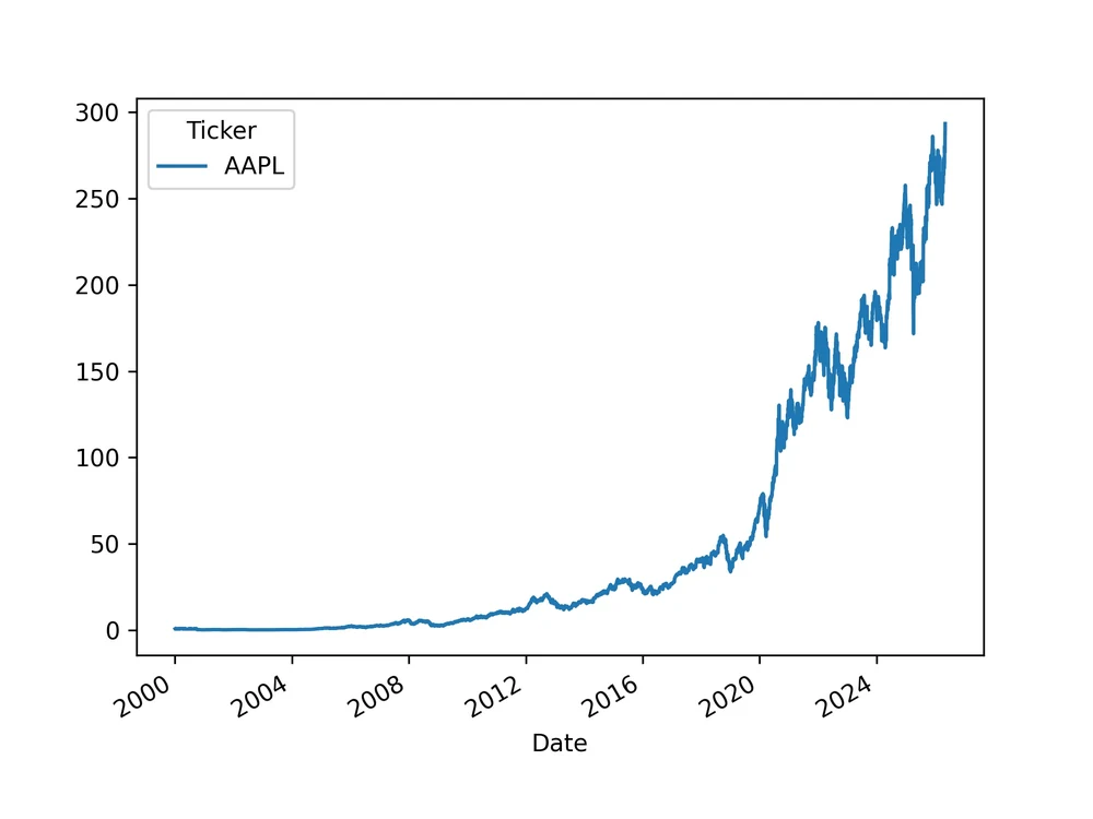
data["Close"].plot() → plt.savefig("chart.pdf", dpi=300)
Plots the 5-year closing price as a line chart and saves it as a 300 DPI PDF. Why PDF? Vector format — scales perfectly for any display or print. The dpi=300 ensures it's print-quality if rasterised.
News Data — What I Explored
I also explored the yFinance news API — not in the final script but in a commented block. The structure is worth understanding because it's your first encounter with nested JSON parsing, which appears constantly in AI API responses:
# This pattern appears in EVERY AI API response
# Learn it now — it will save you hours later

for story in news_data:
    content = story.get('content', {})     # .get() never raises KeyError
    title   = content.get('title', 'No Title')
    summary = content.get('summary', 'No Summary')

    print(f"TITLE: {title}")
    print(f"SUMMARY: {summary}")
    print("-" * 30)
Why .get() matters: story['content'] raises a KeyError if the key doesn't exist. story.get('content', {}) returns an empty dict instead. In production AI systems parsing API responses, missing keys are normal — not exceptions. Using .get() with defaults is a habit that prevents crashes in production.
What I Did NOT Do Today
This is as important as what I did do. It's very easy to go down rabbit holes on Day 1.
- No ML models — that's Phase 2 (Day 11)
- No Pandas deep dive — that's Days 7–8
- No NumPy — that's Day 3
- No advanced OOP, decorators, generators
- No 4-hour YouTube tutorials
- No jumping ahead to LangChain or PyTorch
The roadmap is sequenced deliberately. Everything introduced today — variables, lists, dicts, loops, functions, yfinance — is used in every subsequent phase. Rushing ahead before these are solid creates confusion later.
The Writing Prompt — Why I'm Doing This
The roadmap requires a 1-paragraph writing reflection each day. Today's prompt: "Why does clean environment setup prevent 'works on my machine' issues?"
"When a team builds a financial AI system, every developer, every CI pipeline, and every production server needs to run the exact same code with the exact same results. A conda environment captures everything that makes this possible — Python version, library versions, and dependency trees — in a reproducible, shareable specification. Without it, one developer on Python 3.11 with Pandas 2.2 gets a different result from a colleague on Python 3.10 with Pandas 1.5. In banking and financial services, where model outputs affect lending decisions and risk assessments, 'it works on my machine' is not an acceptable answer. Environment reproducibility is a compliance requirement, not just a best practice."
What I Built by End of Day 1
One honest note: I left a lot of code commented out in day1_stock_project.py — the max/min/mean analysis, daily returns, and plt.show(). That's fine. The point of Day 1 is not to write the most complete script. It's to get comfortable making the environment work, running a real library, and producing a tangible output. The commented code is there to explore tomorrow.
What's Coming on Day 2
Day 2 covers Python OOP + File I/O + Poetry. I'll build a FinancialRecord class that loads the CSV we exported today, stores records as objects, and exposes a summary() method. I'll also set up Poetry — the modern dependency management tool that replaces bare pip for production projects.